Classification--Empirical Study of Heart Disease

Introduction

Heart disease becomes more and more common in our daily life and there are a lot of reasons that are possible to cause it. Here in this simple study, we are going to use classification methods, logistic regression and KNN, to predict whether a patient has heart disease or not.

Click here for the code and data

Data Description

This database comes from Kaggle, which contains 303 data points in total.

Features:

age - age in years
sex - (1 = male; 0 = female)
cp - chest pain type
trestbps - resting blood pressure (in mm Hg on admission to the hospital)
chol - serum cholestoral in mg/dl
fbs - (fasting blood sugar > 120 mg/dl) (1 = true; 0 = false)
restecg - resting electrocardiographic results
thalach - maximum heart rate achieved
exang - exercise induced angina (1 = yes; 0 = no)
oldpeak - ST depression induced by exercise relative to rest
slope - the slope of the peak exercise ST segment
ca - number of major vessels (0-3) colored by flourosopy
thal - 3 = normal; 6 = fixed defect; 7 = reversable defect
target - have disease or not (1=yes, 0=no)

Analysis

Brief Data Exploration

import numpy as np
import pandas as pd
import matplotlib.pyplot as plt
import seaborn as sns
from sklearn.linear_model import LogisticRegression
from sklearn.model_selection import train_test_split
from sklearn import metrics
import os

df=pd.read_csv("C:\Documents\Microeconometrics\Assignments3\heart-disease-uci/heart.csv")
df.head()

	age	sex	cp	trestbps	chol	fbs	restecg	thalach	exang	oldpeak	slope	thal	target
0	63	1	3	145	233	1	0	150	0	2.3	0	1	1
1	37	1	2	130	250	0	1	187	0	3.5	0	2	1
2	41	0	1	130	204	0	0	172	0	1.4	2	2	1
3	56	1	1	120	236	0	1	178	0	0.8	2	2	1
4	57	0	0	120	354	0	1	163	1	0.6	2	2	1

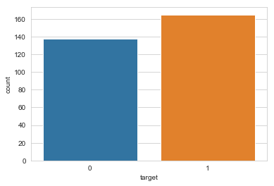
sns.countplot(x="target", data=df)
plt.show()

png

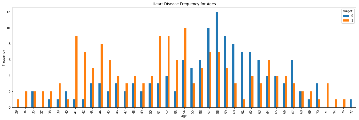
pd.crosstab(df.age,df.target).plot(kind="bar",figsize=(20,6))
plt.title('Heart Disease Frequency for Ages')
plt.xlabel('Age')
plt.ylabel('Frequency')
plt.show()

png

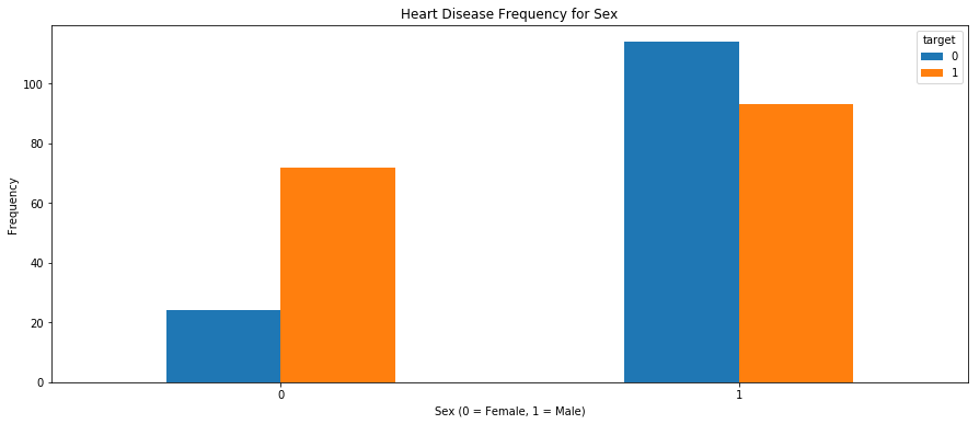
pd.crosstab(df.sex,df.target).plot(kind="bar",figsize=(15,6))
plt.title('Heart Disease Frequency for Sex')
plt.xlabel('Sex (0 = Female, 1 = Male)')
plt.xticks(rotation=0)
plt.ylabel('Frequency')
plt.show()

png

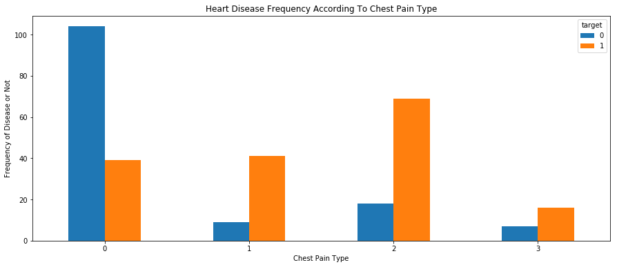
pd.crosstab(df.cp,df.target).plot(kind="bar",figsize=(15,6))
plt.title('Heart Disease Frequency According To Chest Pain Type')
plt.xlabel('Chest Pain Type')
plt.xticks(rotation = 0)
plt.ylabel('Frequency of Disease or Not')
plt.show()

png

Data Transformation

We are going to transform “cp”, “thal” and “slope” into dummy variables for more convenient analysis.

a = pd.get_dummies(df['cp'], prefix = "cp")
b = pd.get_dummies(df['thal'], prefix = "thal")
c = pd.get_dummies(df['slope'], prefix = "slope")
frames = [df, a, b, c]
df = pd.concat(frames, axis = 1)
df = df.drop(columns = ['cp', 'thal', 'slope'])
df.head()

	age	sex	trestbps	chol	fbs	restecg	thalach	exang	oldpeak	...	cp_1	cp_2	cp_3	thal_1	thal_2	slope_0	slope_2
0	63	1	145	233	1	0	150	0	2.3	...	0	0	1	1	0	1	0
1	37	1	130	250	0	1	187	0	3.5	...	0	1	0	0	1	1	0
2	41	0	130	204	0	0	172	0	1.4	...	1	0	0	0	1	0	1
3	56	1	120	236	0	1	178	0	0.8	...	1	0	0	0	1	0	1
4	57	0	120	354	0	1	163	1	0.6	...	0	0	0	0	1	0	1

5 rows × 22 columns

Logistic Regression

y=df.target.values
x_data=df.drop(['target'],axis=1)

#Normalize
x = (x_data - np.min(x_data)) / (np.max(x_data) - np.min(x_data)).values

#Splitting training and testing data
x_train, x_test, y_train, y_test = train_test_split(x, y, test_size=0.2, random_state=0)
logreg = LogisticRegression()
logreg.fit(x_train, y_train)

LogisticRegression(C=1.0, class_weight=None, dual=False, fit_intercept=True,
          intercept_scaling=1, max_iter=100, multi_class='warn',
          n_jobs=None, penalty='l2', random_state=None, solver='warn',
          tol=0.0001, verbose=0, warm_start=False)

y_pred = logreg.predict(x_test)
print('Accuracy of logistic regression on test set: {:.2f}'.format(logreg.score(x_test, y_test)))

Accuracy of logistic regression classifier on test set: 0.87

K-Nearest Neighbor Classification (KNN)

from sklearn.neighbors import KNeighborsClassifier
knn = KNeighborsClassifier(n_neighbors = 5)
knn.fit(x_train, y_train)
prediction = knn.predict(x_test)
print("Accuracy of {} NN Score on test set: {:.2f}".format(5, knn.score(x_test, y_test)))

Accuracy of 5 NN Score on test set: 0.85

# find the best K
scoreList = []
for i in range(1,20):
    knn2 = KNeighborsClassifier(n_neighbors = i)  
    knn2.fit(x_train, y_train)
    scoreList.append(knn2.score(x_test, y_test))
    
plt.plot(range(1,20), scoreList)
plt.xticks(np.arange(1,20,1))
plt.xlabel("K value")
plt.ylabel("Score")
plt.show()

print("Maximum KNN Score is {:.2f}".format((max(scoreList))))
print("The best K is 3, 7 and 8")

png

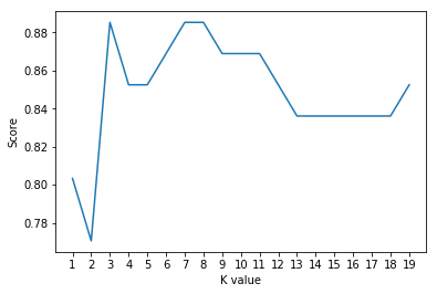
Maximum KNN Score is 0.89
The best K is 3, 7 and 8

Comparing the Two Models

#Accuracy
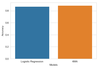
methods = ["Logistic Regression", "KNN"]
accuracy=[0.87,0.89]

sns.set_style("whitegrid")
plt.ylabel("Accuracy")
plt.xlabel("Models")
sns.barplot(x=methods, y=accuracy)
plt.show()

png

#Confusion matrix
from sklearn.metrics import confusion_matrix

y_head_lr = logreg.predict(x_test)
knn3 = KNeighborsClassifier(n_neighbors = 3)
knn3.fit(x_train, y_train)
y_head_knn = knn3.predict(x_test)

cm_lr = confusion_matrix(y_test,y_head_lr)
cm_knn = confusion_matrix(y_test,y_head_knn)

plt.figure(figsize=(15,6))
plt.suptitle("Confusion Matrixes",fontsize=24)
plt.subplots_adjust(wspace = 0.4, hspace=0.4)

plt.subplot(1,2,1)
plt.title("Logistic Regression Confusion Matrix")
sns.heatmap(cm_lr,annot=True,cmap="Blues",fmt="d",cbar=False)

plt.subplot(1,2,2)
plt.title("KNN Confusion Matrix K=3")
sns.heatmap(cm_knn,annot=True,cmap="Blues",fmt="d",cbar=False)

plt.show()

png

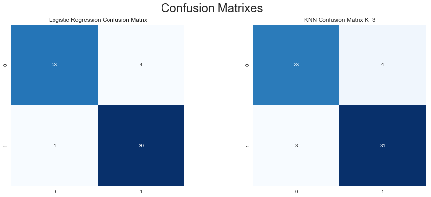
According to accuracy and confusion matrix above, we can see that both models work well with the data but KNN is slightly better. Therefore, we choose KNN (K=3) as the final model to predict if a patient have heart disease or not.

Reference

Building A Logistic Regression in Python, Step by Step

Heart Disease - Classifications (Machine Learning) in Kaggle

Assignment 3