Motivation
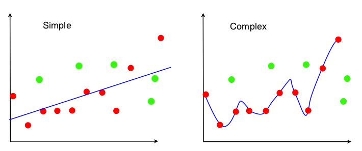
When doing a learning problem, we always want our model to perfectly explain the data, which means that our model not only fits the sample we choose, but also predicts unseen population appropriately. However, it is impossible for us to achieve both goals. Here is an example to intuitively illustrate the dilemma.

For the simple one, although not perfectly fit the sample (red points), it still has some predictive power for the underlying population. The complex one does go through every single point in the sample, but almost lose all explanatory power for the out-of-sample data. We call these two extreme cases underfitting and overfitting respectively.
Bias-Variance Decomposition
To solve the problem mentioned above, we need to first identify those two kinds of errors. Usually we use Mean Square Error to measure the fitness of a model, but it cannot tell us whether the model is overfitting or underfitting.
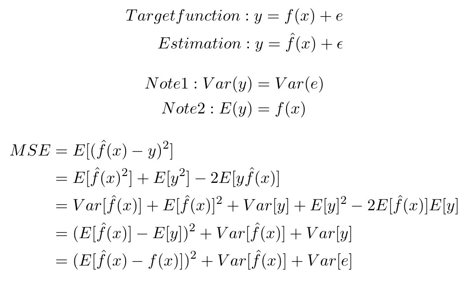
However, there is a way to divide MSE into three parts, called Bias-Variance Decomposition, which is able to identify the two errors. Here is the derivation:
 On the right-hand side of the last line, MSE is divided into the following three parts:
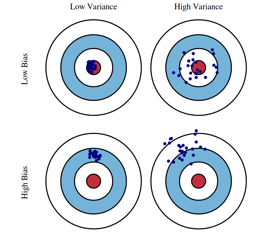
- Bias Error It represents the error due to inability of hypothesis hat f(x) to fit target f(x) perfectly. More specifically, bias suggets how far our estimation away from the target function. If bias error of the model is high, the fitness of in-sample data is bad and the model is underfitting.
- Variance Error It represents the error due to fitting random noise in data. In other words, how much the learning method hat f(x) will move around its mean. If the variance is high, the model can fit in-sample data pretty good but cannot fit out-of-sample data properly, which is useless when we intend to predict the pattern.
- Irreducible Error
It is the intrinsic target noise that cannot be reduced regardless of what model is used. Therefore, bias and variance are what we care about.

Bias-Variance Trade-off
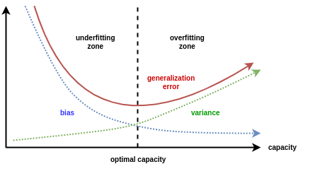
After Bias-Variance Decomposition, it can be mathematically inferred that when bias is close to 0, variance must be very high. Inversely, bias will also be high if variance is close to 0. Therefore, the optimal model should have relatively low variance and bias because in general what we really care about is minimizing overall error.

Limitation and Solution
Bias-Variance decomposition can rarely be calculated, because according to the formula of bias variance decomposition that we derived above, we need to know the actual function to estimate bias and variance, but this is unavailable in the real world for most cases. However, fortunately, to deal with this problem, we can use a resampling technique called \textbf{Bootstrap Aggregating}, in which numerous replicates of the original data set are created using random selection with replacement. Then, each derivative data set is used to construct a new model and the models are gathered together into an ensemble. Predictions based on the ensemble will effectively reduce variance or both bias and variance.
References
Scott Fortmann-Roe, Understanding the Bias-Variance Tradeoff Wiki, Bias–variance tradeoff
For PDF version Click here